
Analogies
In each case in this article, we draw up a circuit, and then show that
it is "equivalent" or "analogous" or isomorphic to some phenomenon or
system. This means that for each electric
quantity in the circuit, there is a corresponding quantity in the other
system
and vice versa. So after we filled in for example "Temperature" for
"Voltage",
we can treat the system using the machinery of circuit theory.
The
principle of Minimum Dissipation
In principle, we can do all circuit analyses with just voltages and impedances. But sometimes it can be handy to introduce extra concepts, and here we want to introduce the concept of the generating functional. (A functional is a formula that produces a number from a set of variables.) The main motivation for this is that in contemporary theoretical physics, the "Principle of Least Action" is considered to be very important. I want to see how this is related to circuit equivalents.
First we will derive an expression for the dissipation in a circuit, and see that the total dissipation is a funky functional.
The set of i equations for a circuit with i vertices:
By multiplying this by 2Vi
,
and summing over all i,
juggling a bit with
indices, we get:
The term (Vj
- Vi)2
/Rij
will be recognized as
the dissipation by the resistor Rij
The theorem we just derived says that the
total dissipation
in a circuit is zero . We can
also see that if Voltage is a
real number, and resistance is a positive real number, as is the case
for "ordinary" circuits, then the dissipation in each component is
positive. This implies that the only solution to a circuit without
sources of energy is that all currents and all voltages are zero. So to
do anything interesting, we have to put in some sources, or consider
putting in as negative or imaginary resistance somewhere.
 A cool property of the total dissipation is that you can recover all
equations
for the circuit by requiring that the total dissipation is in a minimum
with
respect to small variations of
Vi
. Mathematically, this is saying all derivatives to Vi
are zero:
A cool property of the total dissipation is that you can recover all
equations
for the circuit by requiring that the total dissipation is in a minimum
with
respect to small variations of
Vi
. Mathematically, this is saying all derivatives to Vi
are zero:
Which is the original set of equations.
This is why the total dissipation can be considered the generating
functional
of the circuit. Deriving the equations from a generating functional is
not
really adding any new physics, but it is especially useful in seeing
how
different ways of describing things are equivalent.
We call this trick the
principle of minimum dissipation
. It has interesting analogs for the different kinds of circuits I will
discus. For instance in one case it maps onto the principle
of least Action . The principle
of least Action is considered
by some to be the most fundamental principle in theoretical
physics.
The "principle of minimum dissipation" is really a catchy but oversimplifying phrase. It is more accurate to say that all derivatives of the functional with respect to certain state variables are zero. For example, if we had said:
S = ∑i,j Iij2Rij
and then minimize dissipation by varying Iij instead of Vi, we would have obtained:
Iij
= 0
Set up the analogy
:
V(Voltage)
<-> T
(Temperature)
Q
(Charge) <-> U
(Energy)
I (Electric
current) <-> W
(Thermal Power)
P
(Electrical dissipation)
<-> W
ΔT
(see note)
C
<-> ρCp
ΔVolume
(Thermal capacitance of volume
element)
R
(Electrical resistance) <->
Δs2
/(
λ ΔVolume)
(Thermal resistance)
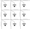
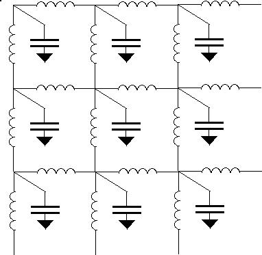
And draw the following circuit :
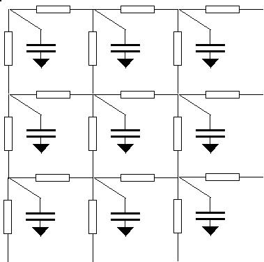
Figure
1: Electric circuit
equivalent for time dependent heat
conduction.
Applying Kirchhoff's current law :
dT/dt
= -1/(ρCp)
div (w) ![]() dTi/dt
= -1/Ci
∑j
Wij
dTi/dt
= -1/Ci
∑j
Wij
Applying Ohm's law :
w
= -(1/λ)
grad
(T)![]() Wij
= -(Ti-Tj)/Rij
Wij
= -(Ti-Tj)/Rij
Combining:
dT/dt
= λ/(ρCp)∇2T![]() dTi/dt
= 1/Ci
∑j(Ti-Tj)/Rij
dTi/dt
= 1/Ci
∑j(Ti-Tj)/Rij
Which is the equation for instationary heat conduction.
Note on irreversibility and the generating functional:
The generating functional of this circuit is:
S
=
∑edges
(ΔT2
/ R)
+ ∑ Vertices
(d/dt
½
C
T2
)
= ∑edges
(W
ΔT)
+ ∑
Vertices (
T dU/dt)
This quantity looks a bit unfamiliar. We know that it should have something to do with irreversibility, because it is the analog of electrical dissipation, the irreversible conversion of electrical energy into heat. It would be nicer if the generating functional were Entropy generation.
Actually, we can do this by switching from Temperature (T) to a quantity that Zemansky called Negcitemp (N=-1/T). According to Zemansky (writer of well known thermodynamics textbooks), it sometimes makes sense to use Negcitemp (Negative Reci procal Temperature) instead of temperature. For small temperature deviations around a nominal temperature, Negcitemp is just like a rescaled temperature. For larger deviations, things get non-linear, but Cp and λ are non-linear functions of T anyway. So let us assume that Cp and λ are linear in Negcitemp, and get for the generating functional:
S
=
∑edgesWΔN
+ ∑Vertices
N
dU/dt
= -∑edges
W Δ(1/T)
- ∑Vertices
(1/T)
dU/dt
= -d/dt
(Entropy)
So now we have the more familiar quantity of entropy generation rate as
the
generating functional, and indicator of irreversibility. This is no big
deal
in practice, but nice philosophically.
 Note that for a right-angled triangle, the "hypotenuse" resistor
becomes
infinite. This means that if we click together 2 right-angled triangles
into
a square, as below, we will retrieve the square schemes as we use in
the
rest of this article.
Note that for a right-angled triangle, the "hypotenuse" resistor
becomes
infinite. This means that if we click together 2 right-angled triangles
into
a square, as below, we will retrieve the square schemes as we use in
the
rest of this article.
 There is a 1-to 1 correspondence between
the metric tensor and the
resistor values for each tetrahedron!
There is a 1-to 1 correspondence between
the metric tensor and the
resistor values for each tetrahedron!
We can
interpret the term as  as
a pseudovector (A*)
whose direction is normal to the (N-1)
simplex built from all vertices except (A)
and whose magnitude |A*|
is
the (N-1)
volume, multiplied by a factor 1/N!.
as
a pseudovector (A*)
whose direction is normal to the (N-1)
simplex built from all vertices except (A)
and whose magnitude |A*|
is
the (N-1)
volume, multiplied by a factor 1/N!.
 The
N-simplex equation.
The
N-simplex equation.To derive
it, we refer to the picture below, again using 3D, but
implying generalisation to other dimensions.
 ,
while
keeping all other lengths constant. This means that the shape of the 2 (N-1)
simplices A*
and B*
cannot change,
and the motion of A and B will be parallel to our projection plane. We
split
the squared length ()
into a component in the projection plane (
,
while
keeping all other lengths constant. This means that the shape of the 2 (N-1)
simplices A*
and B*
cannot change,
and the motion of A and B will be parallel to our projection plane. We
split
the squared length ()
into a component in the projection plane ( )
and a
component orthogonal to it (
)
and a
component orthogonal to it ( ):
):
We expand the
volume into a base |B*|
and height (hb),
and
relate this to the angle (θ):
Write (∂hb
/∂θ)
in terms of A*
and B*:
 ),
we use the cosine law:
),
we use the cosine law:
 :
:
Finally, we
reach QED:
The N-simplex
equation allows us to get the
resistance values from the inverse Cayley Menger matrix:
 Interestingly,
these can be used
to represent higher order
approximations
of continua. Below is a circuit that connects neighbours and
(neighbours)2.
Interestingly,
these can be used
to represent higher order
approximations
of continua. Below is a circuit that connects neighbours and
(neighbours)2.


 It
equals the rate of decrease of capacitive energy.
It
equals the rate of decrease of capacitive energy.Acoustic fields works like heat conduction, but now the resistors are replaced by induction coils. Acoustic fields are reversible, they have no resistors. The requirement that the total dissipation is zero no longer requires that there is a source of energy to have non-zero solutions, because the argument depended on the resistances being always positive; they are now imaginary. These sourceless non-zero solutions are of course: waves!
Set up the analogy :
V
(Voltage) <-> p
(Pressure)
I
(Current) <-> vΔA
(Volume flux)
P
(Electrical power) <-> P
(Acoustic power)
C
(Capacitance) <-> ΔVolume/(κp0)
(Acoustic impedance of a volume)
L (Inductance) <->
ρ(Δs2)
/ΔVolume
(Acoustic impedance of an incompressible duct)
Applying Kirchhoff's current law , and dividing by Ci:
dp/dt
= -κp0/ρdiv(ρv) ![]() dpi/dt
= -1/Ci
∑j(vΔA)ij
dpi/dt
= -1/Ci
∑j(vΔA)ij
Applying Ohm's law across an inductor:
d(ρv)/dt
= - grad(p) ![]() d(vΔA)ij/dt
= -(pi-pj)/Lij
d(vΔA)ij/dt
= -(pi-pj)/Lij
Combining:
On the left sideof the above equation is the acoustic wave equation, with c2 = κp0/ρ. The right side is its discrete counterpart.
As an interlude to all the equations, an animated GIF of an acoustic circuit in one of its eigenmodes:
S = d/dt
∑edges
( ½mv2
) + d/dt
∑vertices
(
½Cp2
)
= d/dt
(total energy
stored in components)
To retrieve the field equations
from this generating
functional, it is probably nicel to use space
time diagrams,
in which
the the principle of minimum dissipation is replaced by the principle
of least Action.
The acoustic equations can be modified to also include terms to account for the transport or advection of inertia, and for viscosity. This leads to the Navier Stokes equation, which describes fluid dynamics. Fluid dynamics is non-linear, and has funky features like pseudo unpredictability.
The central idea for transforming the linear circuit theory to the non-linear stuff like Navier Stokes, is what I call a bucket The idea is shown below.
Figure 3: Principle of bucket discretisation of advection.
After each time step, the fluid will be displaced relative to our cell
structure.
So we have to redivide the fluid among the cells each time step. We do
this
by interchanging buckets. It can be seen from the drawing that the
interchanged
bucket size is vA
dt.
The
buckets carry with them all information of the fluid, i.e.
all dynamical variables such as v,
p,
T,
etc.
It is possible to view this process as a coordinate transformation from
material coordinates,
which are attached to the
fluid, to spatial coordinates,
which are fixed in
space.
Suppose at time t,
we had a cell (i),
which has buckets leaving to a set of neighbours (j)
with volume velocities vij
Aij,
and had incoming buckets from a
set of cells (k)
with volume velocities vki
Aki
. By bookkeeping an arbitrary
dynamic variable (φ)
in the cell, we get:
Which is the discrete version of the advection term in fluid dynamics:
dφ/dt = -(v.∇)φ + ...
The central non-linearity comes from the fact that v itself is also advected:
dv/dt = -(v.∇)v + ...
A good thing about the buckets is that it automatically takes care of some nasty subtleties regarding discretisation schemes which can easily cause numerical instability. (For example, the direction of the flow influences the way we treat a neighbour) The simulation software I made using the bucket idea turned out to be very robust.
We will symbolize the advection
by a bucket drawn at each edge. We then get a diagram for the
compressible
Navier Stokes equation.
Figure
4: Electric circuit
equivalent of the Navier Stokes
equation for compressible fluid dynamics.
The Navier Stokes equation can be further refined by including viscosity.
Here is a cool picture of a Von
Karman Vortex street,
made
with a simulation
based on the modified acoustic equivalent.
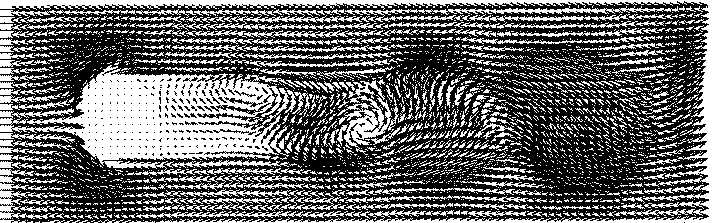
Figure
5: Simulation result of Navier Stokes: A Von
Karman vortex street
Navier stokes on an arbitrary trianglular net
When we try to implement the Navier Stokes equaiton on an arbitrary triangular network, we encounter an additional difficulty. We can use the previously found methods to find all the impedances, and use the bucket formula to transport properties from vertex to vertex. But what is the momentum that we should assign to a vertex?
I have just about finnished writing an article on this, in which I think I figured out how to do it.An interesting network is that below, which turns out to be an equivalent of the Klein Gordon equation.
![]()
The Klein Gordon equation is
the relativistic wave equation
for spin zero particles. The network is drawn for one dimension (x),
and with two layers, UP an DOWN. We derive:
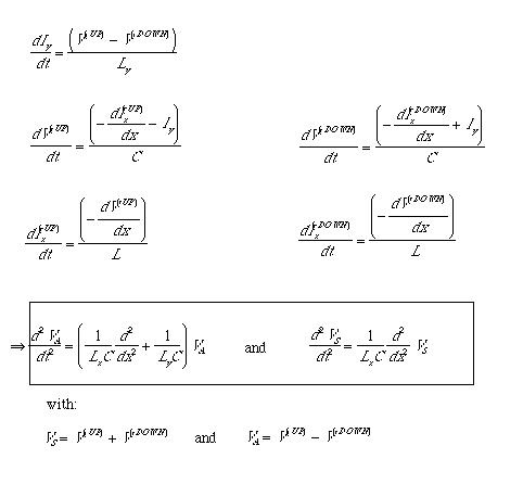
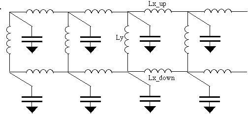
Figure
6: Electric circuit
equivalent of the Klein Gordon
equation, with 2 possible modes.
The equation splits into two superposed modes, the symmetric ( UP+DOWN) and (UP-DOWN). The two modes both obey the Klein Gordon Equation. The symmetric mode has mass zero, and the anti symmetric mode has mass (Ly C)-1/2 . Jos Bergervoet has suggested a simpler circuit for the Klein Gordon Equation:
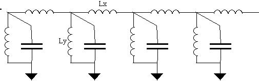
The equation for this circuit is:
It only has one mode (particle
species) as opposed to the previous
circuit, which had 2 modes.
Set up the analogy
:
V
<-> V;
ΔxV
(Voltage
difference in x-direction) <-> -
Ex
Δx
(Chunk of Electric field)
Q
(charge) <-> Q
(charge)
I (current) <-> d(DΔA)/dt
(rate of change of dielectric displacement through surface)
Cx
(Capacitance placed in x-direction)
<-> ε
ΔVolume/Δx2
(Storage container of Electrostatic field energy)
Figure
8: Electric circuit
equivalent for electrostatic fields
Kirchhoff's current law:
d/dt
(div(D))
= 0 ![]() 0 = ∑j(d/dt
(DΔA))ij
0 = ∑j(d/dt
(DΔA))ij
Ohm's law:
D = -grad(V)/ε![]() (DΔA)ij
= -1/Cij
(EΔs)ij
= -1/Cij
∑ij(Vi-Vj)
(DΔA)ij
= -1/Cij
(EΔs)ij
= -1/Cij
∑ij(Vi-Vj)
Combined, this gives:
d/dt
(∇2V/ε
) = 0 ![]() d/dt(-1/Cij
∑ij(Vi-Vj))
= 0
d/dt(-1/Cij
∑ij(Vi-Vj))
= 0
Usually, you say that at t=0, the divergence of the field is equal to the charge density. You then get:
∇2V = ρ/ε
Kirchhoff's voltage law gives:
The Generating functional is:
S = d/dt ∑(E.D ΔVolume)
E.D is the field energy density.
To retrieve the field equations from the generating functional, we have to write it in terms of Vi:
S = d/dt ∑ij ( ½Cij (Vi-Vj)2 )
Comment
on E
versus D
It can sometimes seem a bit irritating to have 2 different quantities
associated with electric fields (E
and D
). In principle, this can be avoided, just like it can be avoided to
use
currents by always writing them as a voltage difference divided by a
resistance.
But I think it is important to distinguish between 1-chunks like Ex
Δx
and (N-1)-chunks
like Dx
ΔVolume/Δx
. This distinction is analogous to the distinction between electric
potential
and electric current, a distinction that we would surely want to be
aware
of when we repair household electra.
Comment
on field energy
This representation may seem somewhat artificial, the vacuum is
supposed
to be empty, and not contain any capacitors. However, the vacuum does
contain
electrostatic energy, which is stored locally in the vacuum. This
energy
is the same energy that is stored in the imaginary capacitors. So they
are
not that abstract as it seems: the energy is really there.
Putting
in conductors
You just put resistors in parallel to the capacitors. Interestingly,
short-circuiting
capacitors increases the capacitance of a geometry, thereby also also
decreasing
the effective speed of light through the geometry. This can be seen
easiest
in one dimension. Suppose a number of capacitors are connected in a
chain.
From Kirchhoff's
voltage law it follows that when
impedances are in series,
you get the effective impedance
of the chain by adding the individual impedances. This means that the
for
the effective capacitance (Ceff): 1/ Ceff = 1/C1 + 1/C2 + 1/C3 + ... If
we
short-circuit some capacitors in the chain, the reciprocal of the
effective
capacitance gets smaller, so the effective capacitance itself gets
bigger.
The
Maxwell equations
The Maxwell equations describe both electric and magnetic phenomena,
and
their interaction. So this is stuff that you need to understand if you
want
to understand nature. To put Maxwell into a circuit diagram, you start
with
the diagram for electrostatic
fields . Then, we have to think
how we can put in the
magnetic field. We think
naturally of inductors, as they seem to be the magnetic counterparts of
capacitors.
But it is a bit tricky. We know that the vacuum does not conduct
electricity,
so we can't put any inductors in parallel with the capacitors. We could
try
putting them in series. But that would mean that there is only magnetic
energy
when a current is flowing through the inductors, and therefor also
through
the capacitors. But this would charge them up indefinitely, and produce
infinite
electrostatic fields. The clue comes from the observation that an
inductor
is not 'elementary', when you look at its geometry. It consists of a
coil,
a spiral of wire. The elementary object is a single loop. After a
considerable
struggle with this idea, I realized that a proper treatment requires a
new
concept, the
mesh inductance. This is an
inductance associated with a loop
rather than an edge.
Generalizing
a circuit to an N-complex
This idea is part of a cool generalization of a circuit,
called a N-complex, or
cell complex. A
conventional circuit can be thought of as a 1-complex. The idea will be
brought along from the following list:
0- Complex : a set of loose
Vertices (points) or 0-chunks
1- Complex: (=Concentional circuit): Edges (or 1-chunks) that connect
Vertices
2- Complex: Faces or 2-chunks that connect Edges
3-Complex: Solids or 3-chunks that connect Faces
N-Complex:
N_chunks
that connect
(N-1)
chuncks
So how do we generalize Kirchhoff's laws and Ohms law? We first need the concepts boundary and the coboundary operators. Boundary and co-boundary operators are just mathematical formalizations of what we intuitively understand right away from the diagrams. Roughly, the boundary of an n -cell is the set of [n-1] cells that form its boundary. The (co)boundary operator will also take care of some minus signs book keeping, associated with the orientation choices of the positive directions.
Suppose we have N
vertices and M
edges. Then the Boundary
operator for Edges can be thought of
as an ( N
X M)
matrix({
aij}),
that has entry aij=0
if the vertex (i)
is not connected to the edge (j),
aij
= -1 if it is the source of the
chosen arrow on the edge, and
aij
= +1 if it is the destination of the chosen arrow on the edge. The
arrows
can be chosen arbitrarily, but once chosen, we should of course keep
them
fixed.
The coboundary of the set of k-chunks
gives the set
of k
+1 chunks that has the k-chunk
as a part of its boundary, once
again taking care of all minus
signs
and arrow orientations etc. The Coboundary matrix for the Vertices is
simply
the transpose of the Boundary matrix for the Edges.
Reformulating
a conventional circuit (1-complex) into
our new jargon
Now we are armed to formulate ordinary circuits in a new jargon, which
will be useful when we start to generalize further.
Step 0. We define a voltage (Vi) on each Vertex.
Step 1. We let the Coboundary operator act on the Vertices (as the discrete analog of the differential Grad operator) producing a set of 1-chunks:
Coboundary (Vi) = ΔVij (Step 1)
This is familiar, we just take the voltage difference across each edge.
Step 2. We apply Ohm's law to to map our 1-chunks to twisted N-1 Chunks:
Iij
= ΔVij/Rij
(Step 2, or Ohms law)
In 3 dimensions, a chunk of current will scale with area. In N dimensions, this generalizes to a N-1 dimensional subspace. Such a subspace will generally have an arrow associated with it. In the case of a surface, we think of the normal vector of the surface.
So why is the chunk called "twisted"? This is because its arrow direction is always inherited from the voltage difference, rather than from its own geometry. Another way to see this is that the spatial information contained in the resistance value Rij is stripped of its arrow; it is always positive. So Iij always has the same arrow as ΔVij. And, if you take the product Iij ΔVij you get an N-chunk of generating functional, which has an always-positve volume associated with it, in contrast to an oriented volume that non-twisted chunks would produce. When we study the Dirac equation, we will put step 2 and 3 together to form the twisted coboundary .
Step 3: Generalize Kirchhoff's
current law.
Coboundary(Iij) = 0 (Step3, or the generalized Kirchhoff's current law)
It may seem a bit strange at first that we use the coboundary rather
than
the boundary. After all, vertices are the boundary of edges. But in
step
2 we made currents N-1
chunks, and the coboundary
of N-1
chunks should be a set of N
chunks. These N
chunks are just the dual of the
0-chunks on the vertices. See figure 9 for an illustration.
Once again, there is an analog differential operator, this time the div operator. Kirchhoff's current law is always about incoming fluxes that have to add up to zero.
Figure
9: Structure of the laws
of electric circuits in terms
of coboundaries.
Combining Step 1,2 and 3, we find the set complete of equations for a 1-complex:
Coboundary(Ohm(Coboundary(Vertices)))=0
What about Kirchhoffs voltage law? We already have a complete mathematical description of the circuit, so the voltage law can be viewed as an alternative formulation. It reads:
Coboundary (ΔVij) = 0
or combining with a previous formula:.
Coboundary (Coboundary (Vi)) = 0
This can be derived directly from the general theorem that the Coboundary of a Coboundary is zero. (Also the Boundary of a Boundary is zero ). These 2 statements are important fundamental laws. They can be visualized if you play around a bit with circuits and arrows, perhaps writing out the boundary matrix.
Note:
The div,
curl and
grad operators
are all instances of Cartan's
exterior derivative (d).
Thus, the
Coboundary operator is the discrete analog of Cartan's exterior
derivative. Ohm's law is the discrete analog of the Hodge
star
operator , multiplied by a
material constant.
Formulating
the Maxwell circuit as a 2-complex
For Maxwell the electric field on an edge can no longer always be
expressed
as a gradient of a potential. This is typical of a 2-complex. So we do
not
start by defining a potential of vertices, but 1 dimension
higher:
on the Edges. This is the diagram:
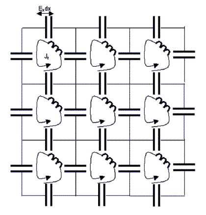
Figure 11: Electric circuit equivalent of the Maxwell equations
With the analogy :
V
<-> V
(Voltage)
ΔxV
<-> ExΔx
(Chunk of Electric field)
Q
<-> Q
(charge)
Jz
(Mesh current)
<-> HzΔz
(Chunk of Magnetic field)
Cx
<-> ε
ΔVolume
/Δx2
(Storage container of Electrical field energy)
Lz
<->μ
Δz2
/ΔVolume
(Storage container of Magnetic
field energy)
Step 0: Each edge has a 1-chunk
EΔs
associate with it, that we call an E-chunk.
Step 1: Take the coboundary of the set of E-chunks. This will give you a set of loops. Note also that there are many different loops that we might want to choose, that all traverse the circuit. We could even in principle choose loops that go round a track 10 times. But the only physically relevant loops are those that we give a finite mesh impedance. In our Maxwell diagram, only the loops that are inside the faces of the cubes have finite impedance and are used. It will be convenient for later to ignore loops that will not get a finite impedance.
Anyway, after taking the coboundary of the E-chunks, we will have performed the discrete analog of curl(E).
curl(E)
= -d/dt
B ![]() ∑along_loop
EΔs
= -d/dt(BΔA)
∑along_loop
EΔs
= -d/dt(BΔA)
We will use this as a
definition of B,
or
magnetic induction. The d(BΔA)/dt
are 2-chunks, that we will call B-chunks.
Step 2: Apply Ohms law, but now use the mesh inductance to map the B-chunks which are 2-chunks onto twisted N-2 chunks, which we define as H. In 3 dimensions, H comes in twisted 1-chunks of HΔs, or vectors associated with a loop. The vector will be recognized as the normal vector of the loop. The equation is the discrete analog of:
H
= (1/μ)
B ![]() BΔA
= 1/Lmesh(HΔs)
BΔA
= 1/Lmesh(HΔs)
Step 3. Take the Coboundary of the H-chunks.
curl(H)
= dD/dt![]() ∑along_loop
HΔs
= d/dt(DΔA)
∑along_loop
HΔs
= d/dt(DΔA)
Step 4. Once more apply Ohms law, but now over the capacitances at each edge, we get the discrete analog of:
E
= (1/ε)
D![]() EΔs
= 1/C(DΔA)
EΔs
= 1/C(DΔA)
Summarizing, we have the Maxwell equations:
curl
(E)
= -dB/dt
H
= (1/μ)
B
curl(H)
= dD/dt
E
= (1/ε)
D
Application of the generalized Kirchhoffs Voltage law by taking the coboundary of the coboundary of E and H :
d/dt
(div(D))
= 0
d/dt
(div(B))
= 0
It is generally axiomized that at t=0, we have:
div
D =
ρ
div
B = 0
Note that we can have magnetic energy without having to charge the capacitors. For example, a constant magnetic field would correspond to identical mesh current in each loop. This means that the net edge currents are zero, so the capacitors are not being charged. The magnetic energy is stored inside the mesh inductance. Once again, this energy is real in the sense that it is locally present in the vacuum.
The Maxwell equations can be combined to form the electromagnetic wave equation:
The model presented for the Maxwell equations could be seen as an aether model . In the link, it is argued that this does not violate relativity.
Putting
in conductors
This is the same as with electrostatic fields, you just put resistors
in parallel to the capacitors.
Putting
in compact components
Sometimes components much smaller than a wavelength can influence the
field.
This is especially the case with resonators. They can resonate at a
frequency
much lower than the frequency that is associated with c/s . (s is a
typical
dimension of the system) To put in these components, you just add them
to
the circuit. You don't have to create the whole geometry, you can just
put
a big physical capacitance across a small 'vacuum' capacitor, which
will
then become negligible. Likewise you can put in coils, not a spiraled
conductors
but as single circuit elements. Then you can start to calculate how
this
physical circuit would interact with the vacuum.
Visualizing the
dynamics:
To visualize an electromagnetic wave, you can picture a line of
capacitors
being charged at time=0. Along this line you would have a constant
E-field,
pointing along the line. This causes a voltage difference across
neighbouring
parallel lines of capacitors. This causes a current to flow,
discharging
the first line of capacitors, and charging the neighbouring ones. But
this
current corresponds to mesh currents. So as the neighbouring E-field is
being
built up, some of the energy is being transferred to magnetic energy in
the
meshes. By the time that the fields of the neighbouring lines are equal
to
the field of the original line, there is no capacitive driving force to
displace
more charge. But now there is inductive driving force, which acts like
an
inertia. The transport of charge continues, now against the direction
of
E. This is similar to a mass/spring system, where the mass will move
against
the force of the spring, once it has gained momentum.
In the meanwhile
capacitive energy is being transferred to neighbours-of neighbours of
the
original line. So the energy spreads out into space. Unlike with heat
conduction, the process is reversible. The
energy is not dissipated, but is pumped back and forth from its
magnetic
form to its electric form.
Animated GIF of a Maxwell circuit. The magnitude of the magnetic field is animated as rate o
Below, an amimation is presented of a Maxwell circuit.
f rotation of the mesh inductors, the magnitude of electric field is animated as the size of the colored bars attached to the capacitors.
The Poynting vector of the electromagnetic circuit is a Cut function: It is assigned to a edge-loop pair. We multiply the 1-chunk of E with the (N-2)-chunk of H to get a (N-1) chunk of power flux (E x H). Note that the Poynting vector in 3D space is represented by more than 3 components in the circuit, which makes it seem unlike a vector. This is because the Cut function becomes only a vector after being "contracted with a cut": If you specify the cut (the analog of a surface), the cut function gives you the flux across the cut at each point.
The Poynting vector as a cut function.
The Generating functional for the Maxwell circuit is:
S = d/dt ∑edges (E.D ΔVolume )+ d/dt ∑ meshes (H.B ΔVolume)
= d/dt ( total energy stored in components)
To retrieve the field equations from the generating functional, we have to write it in terms E only (A form with H instead of E is also possible):
S
= d/dt
∑edges (½
Cedge
(EΔs)2
) +![]() dt
∑meshes
(∑loopEΔs
)2
dt
∑meshes
(∑loopEΔs
)2
But this is more elegantly done
using space
time diagrams
, in which the the principle of minimum dissipation is replaced by the
principle of least Action.
Another important equation in physics is the Schrodinger equation. (It is actually an approximation of the Klein Gordon equation.) It describes the quantum mechanical wave function of a particle in a potential field ( V ).
The Schrödinger equation looks almost the same as the heat conduction equation
. We need to
put in the potential V,
and to take care of i , the
square root of –1. To represent the potential (V),
we add resistors (r)
to ground potential.
The analogy
becomes:
V <->Ψ
1/r
<-> V
ΔVolume
1/Rx
<-> ħ2/(2m)
ΔVolume
/Δx2
C
<-> iħ
ΔVolume
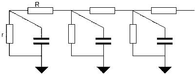
Figure 12: Electric circuit
equivalent of the Schrodinger
equation, with imaginary-valued capacitance.
These together yield the Schrodinger equation, but we had to choose an imaginary capacitance. This is no problem mathematically, we can just do all calculations as we did with real numbers. But it is perhaps a concession to visualizability. A major consequence of choosing imaginary capacitance is that the solutions are now of the type:
Ψ ~ exp(ikx) exp(-iωt)
rather than
Ψ ~ exp(ikx) exp(-t/τ)
A subtle but important difference: It means we don’t get exponential decay with time into thermal equilibrium as with heat conduction but we get everlasting oscillations which conserve |Ψ|2.
Another approach is to try to write out Ψ into real numbers Ψ = ( X + iY ). We then obtain equations for X and Y that are of the form:
d2X /dt2 = d4X /dx4
This equation is like the equation for waves in a bending beam. You can make a kind of beam construction using springs and bars. This has led to a mechanical discrete analog of the Schrodinger equation with springs and rods, that sometimes pops up in literature. I don't know if it can be built using electrical components.
So far, we have considered discrete space, but time has till now been considered continuous. Interestingly, it is possible to construct a model that has space and time discretized in the same way. I like this, because according to the theory of relativity, space and time should be deeply related.
The trick is to put negative
resistance in
the time direction. This sign
is related to the negative sign of the
time component of the metric of space-time.
As an example, we will create
the acoustic wave equation in
terms of a space-time circuit.
We will use the so-called Velocity potential as the analogue
of
Voltage.
Set up the analogy
:
V (Voltage)
<-> φ
(Velocity potential)
Ix
(Electric current in x-direction)
<->(ρvΔAΔt)x
(Mass displacement in x-direction)
It
(Electric current in t-direction)
<-> p
(ρ/(κp0))
ΔVolume
(Pressure times spatial volume)
P (Electrical
dissipation) <-> S
(action)
1/Rx
(Electrical conductivity
in x-direction)
<-> ρΔVolume
Δt
/Δx2
1/Rt
(Electrical conductivity
in t-direction)
<-> -(ρ/(κp0))
ρΔVolume
Δt
/Δt2
Note that (ρ/(κp0))
= c2,
the speed of sound squared.
Figure
14: Electric circuit equivalent of the scalar
wave equation discretized in both space and time.
The velocity potential (φ) is defined such that:
v
= -grad φ
p/ρ
= -dφ/dt
Velocity and pressure live in the circuit as voltage differences across edges (i.e. as 1-chunks):
vxΔx
= -Δxφ
p/ρΔt
=
-Δtφ
Write out Kirchhoff's current law at a vertex (using Ohm's law to get the currents):
(ρvΔAΔt)x[x,t]
- (ρvΔAΔt)x[x-Δx,t]
+ (ρ/(κp0))p[x,t]
ΔVolume -
(ρ/(κp0))p[x,t-Δt]
ΔVolume
= 0
Divide by ρΔVolumeΔt (assumed constant for the moment) and rearrange:
( p[x,t] - p[x-Δx,t] )/Δt = - (1/(κp0)) ( vx[x,t] - vx[x,t-Δt] )/Δx
Which is the discrete analog of:
dp/dt = -(1/(κp0)) div v
Next, write out Kirchhoff's voltage law around a loop:
vx[x,t]Δx
+ p/ρ[x+Δx,t]Δt
- vx[x,t+Δt]Δx
- p/ρ[x,t]Δt
= 0
This time, divide by Δx*Δt/ρ, and rearrange:
( ρvx[x,t+Δt] - ρvx[x,t] )/Δt = -( p[x+Δx,t] - p[x,t])/Δx
Which is the discrete analog of:
dρv/dt = -grad p
So we once more have the acoustic wave equation, but now
in space-time form.
There is now no longer a role for the inductors and capacitors, the only component is the resistor.
The Generating functional
is now
=∑edges
(dφ
/dxμ)(dφ
/dxμ)
ΔVolume Δt
The generating functional is
now Action instead
of dissipation. The "dissipation" in this analogue has of course no
longer anything to do with energy loss.
Action is a fundamental quantity, perhaps even more fundamental than
energy.
In a sense, it is energy density integrated over space and
time.
According to quantum mechanics, there is a fundamental chunk of action,
equal to ħ.
More on that in the future.
Note that the use of negative resistances in the time direction means that the total action (<->dissipation) in the circuit is zero.
We can also put the Klein Gordon equation in space-time form, by connecting a resistance to ground potential to each vertex. The mass term is represented by a current to ground.
Application: The discrete time harmonic oscillatorWe can use the idea
of space time circuits to make a discrete
time harmonic oscillator, a zero dimensional wave
equation.
The harmonic oscillator, with dynamic variables (x,p)
can be represented by a continuous-time
circuit equivalent:
We can write down dynamic equations to get from time (t) to time (t+1):
The system has an exact solution:
I believed for a while that
space time circuits do not have
solutions
that conserve energy in the time direction, but I was pleased to find
that actually they do: The eigenvalues of
the dynamic
equations are complex conjugates with unit magnitude, as long
as  .
(Remember Rx is negative)
.
(Remember Rx is negative)
The dissipation in the resistors represents chunks of Action:
Energy times
time-interval.
Space-time circuit for the Maxwell equations
In the diagram below, we apply
the idea of a space-time
circuit to the
Maxwell equations. It all works out nicely, and we obtain the
relativistic
formulation of the Maxwell equations in terms of the 4-vector potental (A)
and field tensor (F).
Figure
15: Electric circuit equivalent of the Maxwell
equation discretized
in both space and time. To depict it in 3D, we draw only 2 dimensions
of
space.
The capacitors and mesh
inductors are replaced by mesh
resistances. Like
in the scalar case, the dissipation in these resistors is reinterpreted
as
Action. Again following the scalar case, the mesh resistances which
have a time component (Rtx,
Rty,
Rtz)
are negative, so that
the total action in the circuit is zero even with non-zero currents.
We do not use a scalar potential φ,
but
a vector potential A,
a 1-chunk of which (AμΔrμ)
is defined on each edge. In (3+1) space-time dimensions, there are 4
components of A
, and 3+3 components F.
The 3+3 components
of the electric
field and the magnetic field are now contained in the 6 mesh F-chunks FμνΔrμΔrν.
Lets remind ourselves of the
relation between F
and A,
and their more familiar friends E
and B:
Fxy
= dAx/dy
- dAy/dx
= Bz
Fzx
= dAz/dx
- dAx/dz
= By
Fyz
= dAy/dz
- dAz/dy
= Bx
Fxt
= dAx/dt
- dAt/dx
= Ex
Fyt
= dAy/dt
-
dAt/dy
= Ey
Fzt
= dAz/dt
- dAt/dz
= Ez
or, using 4-index notation:
Fμν
=
dAμ/drν
-
dAν/drμ
![]() FμνΔrμΔrν
= (dAμ/drν
- dAν/drμ)ΔrμΔrν
FμνΔrμΔrν
= (dAμ/drν
- dAν/drμ)ΔrμΔrν
The mesh resistances Rμν:
Rμν = εμν (ΔrμΔrν)2 / (ΔVolume Δt)
The Generating functional is now the Action of the electromagnetic field:
S = ∑meshes (ΔμνA)2 /Rμν
Note the compactness of the relativistic formulation of the Maxwell equations.
If we impose Kirchhoffs current law on A, we get the discrete version of the Lorentz gauge condition dμAμ = 0.
With electric networks, you can
implement any
metric of space time. If dx,
dy,
dz
and dt
vary from place to place, as in curved space, you can just adapt the
impedance
values accordingly. Furthermore, there is a 1-to-1 correpondence
between the metric tensor in a simplexial chunk of space time and the
resistors on its edges, as we saw in the section on the N-simplex equation.
You could reinterpret the
changes values as being
caused
by a variable ε
and μ
constants of the vacuum. There are even people who tried to construct a
gravity theory on this principle, for example:
http://arxiv.org/abs/gr-qc/9909037
A link brought to my attention by Gordon D. Pusch.
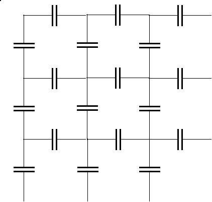
Relation of circuit analogies to bond graphs
Like electric circuit analogies, Bond graphs are a way to model all kind of things in a unified way. The bond graph aproach is more or less equivalent to the electric circuit analogy approach. Below is a model of a 2D acoustic medium in both bond graphs (red) and electric circuit (black). Bond graphs also use pairs of variables whose product is power. The voltage-like quantities are called "effort", and they are located at nodes labeled "0". These nodes also imply Kirchhoffs current law for the other, or "flow", variable. The "flow" variables can be thought of being located at the "1" nodes, on which Kirchhoff's voltage law is implied. The arrows are interpreted as flows of power, or "Power bonds". The bonds go from "0" and "1" nodes to element nodes. These elements force an equation between effort and flow, just like circuit elements. Note that in the diagram below a 1-node is used to create a voltage difference, which is then coupled to the inductance L.
Bond graphs are often used in models whith multiple domains, for examplea loudspeaker, whic has an electric part and a mechanical part. A similar transfer between elctrical and mechanical domains is possible with electric circuit equivalents, using a transformer. A purely electric transformer has a dimensionless winding ratio, but we can give it a dimension, to convert from voltage/current to for example velocity/force.
A transformer can interface between different physcal domains, eg from elctric to mechanical.
Eric Forgy has drawn my
attention to some links and literature
on related subjects. A good start is here:
http://math.unm.edu/~stanly/mimetic.html
I missed some of this literature previously, because different key
words
are used. For example I had never heard of Hodge star, co-boundaries,
etc.
(My excuse is that I am an engineer, normally working on very different
things)
A keyword is "mimetic" which means that a discrete system mimics a
continuum.
The keyword "cell method" refers to a discretisation method that is
much
like a circuit mathematically, but uses different symbolism. I have
tried
to learn the lessons from some of this literature, and incorporate it
into
this page.
Another place where I learned a lot is this newsgroup:
sci.physics.reseach (Google archives all messages)
And a new group, focussing on discrete physics:
sci.physics.discrete (Google archives all messages)
Further work on electric circuits.
New results will be published when available. Specifically, I am thinking of: