Solar eclipse effect on the propagation of LF radio signals.
Written by M. Sanders, PA3BSH.
Revision 1a, may 1st. 2001. (reference update on URL)
INDEX:
APENDIX A: Measurement method.
Copyright.
1 Summary.
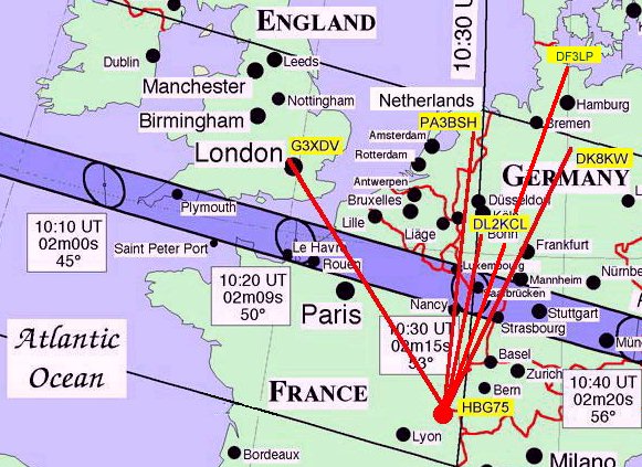
During the 1999 solar eclipse on august 11th. a group of European Radio Amateurs have measured the signal strength from various LF, MF and HF transmitters. This report is based on the observations of the radio time signal transmitted by the Swiss station HBG75. The shadow from the moon passed between the transmitter and observation points in England, Germany and the Netherlands.
All observations show a distinctive change in signal strength around the time the eclipse passes the propagation path between the observation points and the HBG75 transmitter. The observations are different from propagation under normal conditions when usually only slight variations in signal strength occur.
There are 4 distinctive types of signal change behaviour during the solar eclipse. There is a relation between the frequency of the signal observed and type of behaviour as well as., the amount of signal change. The propagational distance and bearing between the transmitter and the observer have a secondary influence on the observations.
The phenomena of signal change at 75 kHz. can be explained by D layer bahaviour and there is a great simulatity between the solar eclipse effect on LF propagation and the propagational behavour during sunrise and sunset. A simuation model was used to evaluate both the solar eclipse measurements and sunset measurements. The results proved the model gives a reasonably accurate output in both cases.
It can be derived from the the model that during the solar eclipse the D layer decreased height rapidly followed by a further decrease of the ionisation index when the shadow of the moon took away most of the suns ionizating radiation in the ionosphere. A relaxation process caused a time delay in the observations of this phenomena. When the solar radiation returned to its original level respectivily the ionisation index and the D-layer height returned to almost the same level as before the eclipse.
Variations in the observations and some anomalities recorded confirm the D layer is not as homogeneous as some popular literature suggests.
2 Observations.
The following HBG75 measasurements have been recorded with the method described in apendix A.:
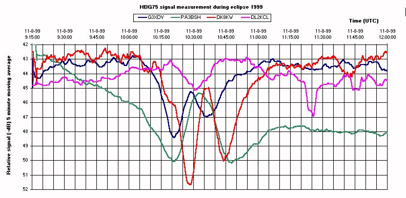
The effects at different observation recorded points can be divided into four groups:
3 Considerations.
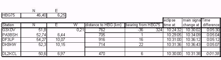
Most observations show no correlation between 'peaks' and 'nulls' and the times of the eclipse maximum at the transmitter site or at the observation point. All observations at greater distances show almost the same time delay of about 5 minutes between the time the eclipse crosses the propagation path and the time when 'nulls' or 'peaks' occur.
Observations show different effects on different frequencies and on signals with different propagation distances. There is no uniform effect recorded when different radio signals are measured at one observation point.
Most measured signals return some time after the eclipse to almost the same level as before the eclipse. Some measurements indicate significant signal level changes between before and after the eclipse. Some W-shape observations show peak levels during the eclipse that are above the level recorded before and after the eclipse.
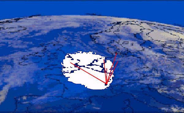
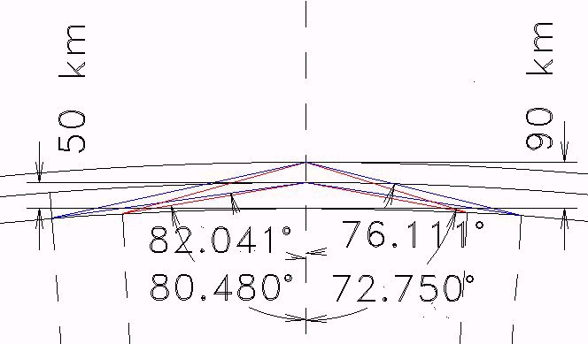
The 'lines of sight' as shown in the chart above are presented as a straight lines. The radio signals propagate along the earth surface following 'great-circles' . There is some deviation between the lines as drawn and the actual propagation paths.
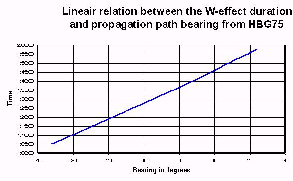
There is a difference in the overall time of the W-shape recorded at the different observation points. The following diagram shows there is a linear relation between the overall time and the bearing of the propagation path from HBG75 as calculated from the geographical coordinates.
The observations done at an observation point at almost the same longitude and within the 90% solar eclipse limit will produce measurements from propagation through 'full darkness'.. Observations done at an angle crossing the solar eclipse line will produce measurements from propagation through partly and fully darkened zones. There does not seem to be a mayor influence caused by this fact.
Satellite images show the eclipse has a shadow circle projecting slightly oval shaped on Europe. The oval moves over England starting shortly before 10:00 hours UTC (UTC=GMT Summertime in England = UTC-1 hour, summertime in Germany and The Netherlands = UTC-2 hours.) .
4 Analysis of the HBG75 measurement data.
OBSERVATION TYPES.
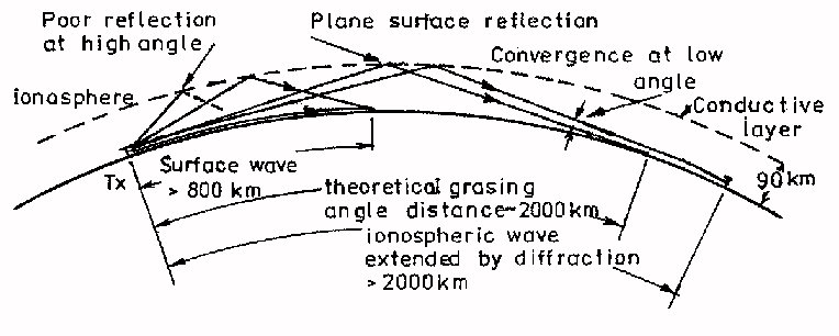
The type 1 observations are made at ground wave propagation distances. It is safe to assume ground wave propagation is not affected by the solar eclipse.
The type 2 effect occurred at observation points just over the horizon. The propagation is surface wave type. This is a mixed mode where groundwave and refraction in ionosphere combine and form a wave front (surface wave) bending along the earth surface.
The type 3 effect was not recorded on 75 kHz.
The type 4 shows a typical 'W-shape' . The distance between transmitter and receiver is over approximately 500km. At thist distance reflection or refraction in the ionosphere become the mayor factor propagating the surface wave. Ground losses have attenuated the original ground wave and only 'virtual' diffractedg hroundwaves are present in the combined surface wave.
LINEAR RELATION BETWEEN BEARING AND OVERALL TIME.
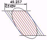
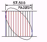
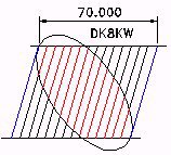
The linear relation between the bearing and the overall time of the recorded type W-shape effects can be explained if the projcection of the moon shaddow is taken into consideratioin. When a circular shape is put into a light source under a certain angle the projection will be an oval shaddow instead of a circular shaddow. Only at a angle of indecence of 90 degrees a circular shaddow will be projected. The propagation paths can be placed onto this oval at regular distances (times). The following diagrams show the effect.
|
|
|
|
This explaines the time difference in the recorded W-shapes at the different observation points.
5 The D-layer and its behaviour during the solar eclipse.
To understand the different observation types it is nescessary to look at the D-layer influence on the propagation of LF radio signals.
CHEMISTRY AND IONISATION.
The ionosphere between 50km and 100km height consists mainly of Nitrogen and Oxygen atoms and the molecules they can form like O
2, N2, NO etc. These atoms and molecules ionise under the influence of solar radiation. According to quantum mechanics sunlight as well as all other electromagnetic radiation consists of fotons (energy packets). The energy of fotons increases with their frequency in the electromagentic spectrum. The Ultra violet light and x-ray's emitted from the sun have ionisating energy levels. Ionisation means an electron from an atom is 'hit' by a foton and absorbes its energy. The electron will leave the atom when the electron reaches an energy level higher than the energy with which the atom can bind it. The atom remains as an positive ion when one or more electrons are missing. The physics of ionizating radiation describe this effect.After a certain time electrons recombinate with ions or atoms. The amount of time is dependent on the probability that free electrons will meet ions, atoms or molecules. This probabiltiy increases with the density of the gas. It is known the density of the Ionosphere decreases exponentially with height. Below a cetain density (above a certain height) the electrons can exist seperatly from ions for a longer period of time. All efects on the propagation of radio signals (electromagnetic radiation) in the ionsophere are caused by the free electrons. The lowest layer of ionisated gas with free electrons capable of influencing the propagation of electromagnetic radiation in the earth ionosphere is called the D-layer.
ELECTRON MOVEMENT IN THE IONOSPHERE.
When observing the phenomena of ionospheric ionisation from a mechanical point of view it is obvious the main flow of fotons is away from the sun and into the ionosphere towards earth. It can be expected most electrons will have a momentum after the colission with a main directional vector towards the earth. A statistical (Gausian) spreading in directions will occur and the earth magnetic field will have its influence but in fact a flow of electrons is pushed down in to the lower ionosphere. Providing the lower part of the ionosphere with relatively more free electrons. This surplus of electrons also moves just below the existing equilibrium caused by the gas density. This effect can be observed as an apparent movement downwards of the D-layer during day-time as a new equilibrium is formed at a lower altitude.
REFLECTION OF LF SIGNALS.
Propagation of radio signals is affected by the ionised layers in the ionosphere. The D-layer attenuates medium, high and ultra high frequency signals passing the layer where the attenuation decreases with an increasing frequency. Radio signals with al long wavelength (Low Frequency) can reflect against the bottom of the D layer. There is a analogy between the physics of light and the propagation phenomena of radio signals. The D layer acts as a partial mirror for LF signals. The amount of reflected energy is described by the reflection coefficient with the follwoing formula:
Xd (-dB) = 0.57 * f(x) * sin(i) * k
Both the angle if indecence (i) and the ionisation index (k) are mayor factors for the amount of reflected energy. It is known that at daytime the apparent D-layer height is about 50 km. and at night the height increases to about 90 km above sea level. A changing D-layer height will change the angle of indecence (i) for the propagation of signals between two fixed points. The ionisation index at night is about 0.5 increasing with the amount of ionisating radiation to about 3 at daytime. The frequency in the formula is given in kHz. Variations in the solar radiation intensity will both affect height and ionisaton index. The following graph shows the Reflection coefficient for an angle i = 80.79 degrees (cos(i)=0.16). The red line is placed at approximately 75 kHz. The influence of the changing ionisation level (Lx) is 16dB (approx. 1:40) between day and night. However after correction for the lower cos(i) at night only a 3-6 dB change in reflected signal strenght can be observed.
OTHER FACTORS.
Ionospheric winds exist with movement paterns like the pasat winds and circulations like the pressure systems in the lower atmosphere . In the analysis of the solar eclipse effect on LF propagation these effects as well as tidal waves formed under the infuence of the attraction of the gasses by the gravity of the moon have not been taken into consideration.
RECEPTION OF LF RADIO SIGNALS.
When signals from a transmitter (Tx) reaches the observer energy from the groundwave as well as the reflected wave induce a current in the antenna. The size of the antenna current is measured by the receiver and is presented in the form of a signal strength readout. The groundwave decreases with increasing distance due to attenuation by the earth surface. The signal strength by the reflected wave is dependent on the reflection coefficient. Therfore the relative influence of the reflection coefficeint ont the overall signal strenght increases considerably with distance.
THE EXPECTED SOLAR ECLIPSE EFFECT ON THE D-LAYER.
The solar-eclipse or moon-shadow takes away a lot of solar radiation and the Ions in the D layer recombinate during the eclipse. The effect is exactly the same as takes place during respectively suset adn sunrise. The difference between sunrise/sunset and the solar eclipse is the angle of solar radiation on the earth. During dawn and dusk the radiation passes almost horizontally through the ionosphere, slowly 'heating-up' or 'cooling-down' the ionosphere, atmosphere and biosphere. The 1999 solar eclipse was observed in Europe around noon when the solar radiation passes almost vertically through the ionosphere. The recombination and ionization during this eclipse took place in a short amount of time compared to sunrise and sunset. The effects on the D layer and the related effects on the propagation of LF radio signals took place in the same short amount of time.
6 A mathematical model for the solar eclipse effect on the reflection coefficient.
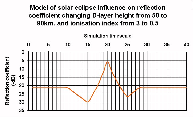
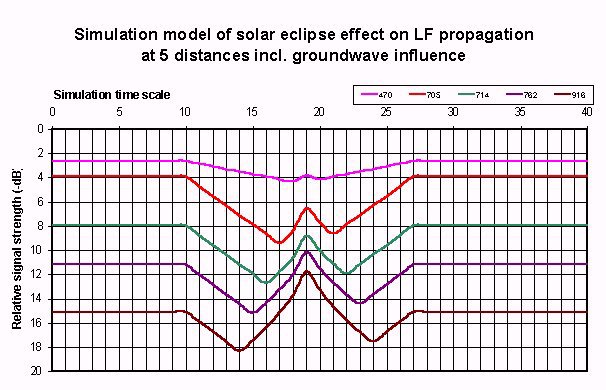
A relatively simple linear mathematical model can be built to test the effects of the solar eclipse on the reflection coefficient at various distances. The output of the simulation is the reflection coefficient at a given distance between transmitter and receiver. The simulation tests the different rates of change in height and ionisation level of the D-layer.
It was only possible to obtain a W-shape from the simulation model if the variation in heigth is set to take place rapidly and immediately at the beginning of the moon shaddow coverage of the propagation path. The decrease in ionisation index apparently takes place later in time and this process is not as fast.
The following graph shows the output of the mathematical model.
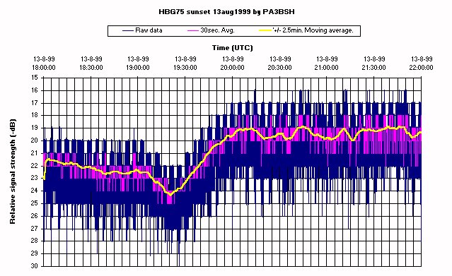
For reference the model was also used to simulate the influence of a sunset on the reflection coefficient. The parameter set obtained from the solar eclipse simulatios was also used for this tests The following graphs show the output of the mathematical model and the measurement results from a reference measurement of the HBG75 signal.
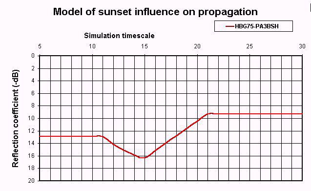
Because of the striking resemblance between all observations and the simulation results it can be concluded that the model gives a reasonably good representation of the actual changes in height and ionisation rates and their effect on the reflection coefficient and thus of their effect on the propagation of LF radio signals.
7 Correcting the model for groundwave signal influence.
The simulation output showed that the absolute changes in signal strenght increase at shorter distances between transmitter and receiver. This is in contradiction to the observations during the solar eclipse. This means there are one or more other factors influcencing the actual changes in signal strenght.
The most obvious factor to be taken into consideration is the ground wave. At greater distances the influence of the ground wave on the actual signal strength decreases exponentialy.
A second factor is the so called cut-back factor. When the D-layer height decreases from 90 km to 50 km height only radio signals transmitted at a verry low angle to the horison reacht the observer. It is known that electrical losses in the earth along the propagation path decrease the signal strength increasingly with lower transmission angles. Therefore at greater distances the D-layer height increase during sunset and the first stages of the solar eclipse will cause a stronger increase of the signal strength than can be explained by the changes in the reflection coefficient alone.
When the model is corrected for the increase of influence at a greater distance the following simulation output is obtained:
These results show that with the help of the solar eclipse measurement data a reasonably accurate simulation model could be built that is also cabable of interpreting measurement data of other signal change measurements. Alle singnal changes can be related to D-layer heights and ionisation rates.
When the changes in heigt are regarded as more or less constantly changing from 50 to 90 km then only the initial ionisation level and rate of change have to be put into the model to fit the simulation curves to the actual measurement data. Therfore it is also possible to give a good estimate of the ionisation rates before, during and after events like sunrise, sunset and the impact of solar flares on the D-layer by fitting the simulation model onto actual measurement data.
8 The 5 minute time difference and relaxation effects.
The difference in the time the eclipse passed the propagation path and the recorded signal changes can be explained by taking the effects of a relaxation process in to consideration. Ionization is a non lineair proces witch only takes place when the ionizating radiation reaches a certain level of intensity. Therefore the recombination starts some time before the solar eclipse passes the propagation path. This relaxation process continues some time after the eclipse 'maximum' causing a further decay of the ionisation level of the D-layer.
With the analogy to other ionisation processes in mind the following basic eqasion for the process can be expected:
K(t=x) = k(a) + k(t=0) *
e -(p*t)Where k(t=x) is the ionisation index at time x; k(a) is the ionisation level at night (background radiation?). Whith data derived from the reflection coefficient model a D-layer p can be estimated to lay be between 1*10
-3 and 2*10-3 . For echt ionospheric height there should be a specific constant p because the density of the gas is the main factor determining the average lifetime of free electons in the ionospheric gas.When looking at the solar-eclipse the moon moves gradually over the sun with the following stages:

The factor k(e) changes with the visible area of the sun during the eclipse. The area changes can be calulated and the results are presented in the following graph:
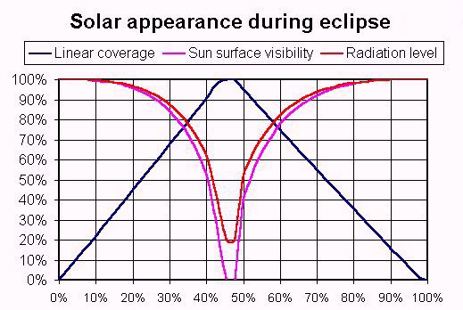
The rate of change is exponentialy increasing near the time of the maximal solar coverage by the moon. Because the signals stenght is measured in a dB scale a more or less linear rate of change will occur as far as changes in the ionisation level are concerned. This linear effect is implemented as far as the simulation model for the reflection coefficient is concerned. The rounding of the signal towards peaks and nulls in the measurement data indicate some linearity that can also be explained by taking relaxation processes into consideration.
9 Anomalities.
Chaos theory and the behaviour of other gasses (water-vapor, ozone etc.) in the earth atmosphere make it hard to believe the layers in the ionosphere are homogeneous. This may account for 'local' anomal observations, measurement variations as well as different effects at different observation distances.
There are several observations indicating a change in signal level between before and after the eclipse. This suggest a change in the reflection coefficient of the D layer since the amount of reflection determines the signal strength of signals propagated at distances over the optical horizon. It is most likely 'clouds' with relative high density exist in the ionosphere. A 'cloud' dissolves with the recombination of the ions and after the eclipse some new 'clouds' have been formed.
There have been more recordings of solar energy change related anomalities in the propagation of LF radio signals. It would be most interesting to study this phenomena and try to locate 'clouds' by correlating signal changes in radio signals with crossing signal paths.
10 Acknowledgments
.I would like to thank the Belgian Amateur Radio society UBA and their project team for the development and distribution of the ON5OO 'Eclipse' software. Furthermore I would like to thank Mike Dennison, G3XDV, Gerri Kinzel, DK8KW, Peter Schnoor, DF3LP and Andreas Tschammer, DL2KCL for their measurements and providing the measurement data.
11 Literature and references:
More information can be found on the Internet at the following sites:
Propagation of long radio waves by J.A. Adcock, VK3ACA published by the Wireless Institute of Australia in Amateur Radio magazine 1991:
http://www.lwca.org/library/articles/lfprop/adcock/lfprop6.htmUBA:
http://www.uba.be/Mike Dennison, G3XDV:
http://www.lf.thersgb.net/gallery/eclipse.htmGerri Kinzel, DK8KW:
http://home.t-online.de/home/dk8kw/hbg75.htmAndreas Tschammer, DL2KCL:
http://www.datelsoft.de/dl2kcl/page4.htmlPeter Schnoor, DF3LP:
ftp://ftp.rz.uni-kiel.de/pub/nephro/nephlab/lp/8-11day.gif
APENDIX A.
Measurement method.
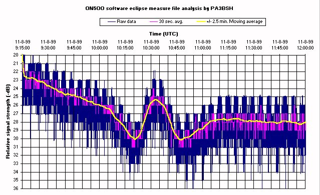
Measurements have been made by recording the audio frequency output of radio receivers. The receivers have been set not to change amplification of the RF/AF signals during measurement (AGC off) . Since amateur receivers are low distortion devices with practically lineair signal amplification all changes in the radio frequency input level can be measured at the low frequency (audio) output of these receivers. The Belgian Amateur Radio society UBA provided ON5OO software capable of measuring the strength of the audio output of a receiver by using a soundcard in a Personal Computer. The signal strength is measured in a logarithmic scale (dB) and logged into a file. The file contains the measurements taken each second together with the time and date. Some measurements have been done with other data acquisition hardware and software and the data has been converted into the ON5OO data format.
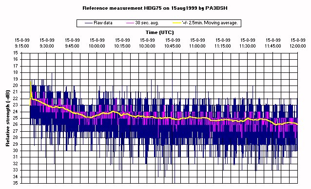
The data measured by the author is shown below. The data shows a strong fluctuation in signal strength forming the broad blue line in the plot. The HBG75 radio station transmits a time signal. The transmitter power is turned on and off in a one second period. This on-off keying is the main cause for the variations of signal strength in the raw sampling data. The ON5OO software also calculates a 30 second average and this data is also plotted in the diagram in purple. A second averaging algorithm was used when post processing the data. This average is shown as the yellow line. Averaging influences the location of signal changes on the time scale in a graph. With a -2,5/+2,5 minute moving average the 'peaks' and 'nulls' appear in the diagram with a minimum effect on the timing of the events.
The following diagram shows a typical reference measurement of the HBG75 signals. Only a slight change in signal strength can be seen.
Copyright.
Copyright HTML page including illustrations M.Sanders 1999, ON5OO 'Eclipse' software UBA 1999. Chart of the eclipse path provided by NASA .
Feel free to hyperlink or refere to my homepage: http://www.xs4all.nl/~misan Unauthorized downloading, distribution, mirroring and modifications are prohibited.
![]()
HTML link to:
Homepage M. Sanders, PA3BSH